A Roadmap to a Continuous Control Strategy

See Per speak on this topic during “Plenary 4: Bridging Current Technology with the Future of Medicine,” March 13, 9 a.m.

Throughout the manufacturing process, there can be risks. In particular, there is a risk of potentially overlooking errors due to uncertainty in estimations if verification is based on sampling. What if there was a way to account for this risk?

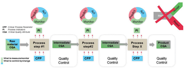
Many pharmaceutical manufacturers are working toward continued process verification per global regulators’ expectations. “Continued” means an ongoing effort after validation, but it can be based on sampling. “Verification” is a passive act; a process is estimated to meet specifications without any adjustment of process parameters. In many cases, however, the current state is continued product verification where product critical quality attributes (CQAs) are tested after processing, similar to traditional batch release testing. The ideal state is to have continuous (always) process verification and control, meaning process parameters are adjusted to ensure processes remain on target. Figure 1 depicts the ideal state. Here, each unit operation is continuously monitored, and actions are taken if quality standards are not expected to be met.

This requires three improvements to continued product verification: 1) process verification for early feedback with easier identification of causes, 2) continuous verification to corroborate the process, and 3) process control by using measured process signals as a criterion for changing process settings.

When moving to a continuous process control approach, three questions must be answered.

1. What to monitor?
2. When to act?
3. How to act?

1. What to Monitor?

Real-time monitoring requires a series of process indicators (PIs) that can be measured in real time and correspond with the CQAs. Typically, determining CQAs needs a set of PIs. Often, the critical settings of the process, i.e., critical process parameters (CPPs), are also included in predictive models for transfer function F:

Predicted CQA=F(CPP₁,…CPP_n ,PI₁…PI_m)

Next, the relationship between PIs, CPPs and CQAs must be established. The recommended procedure involves performing a design of experiment (DoE) that systematically varies CPPs. CQAs and PIs are then measured as responses. By conducting a DoE with uncorrelated CPPs, a relationship between CPPs and CQAs and/or PIs is due to a casual effect. In addition, this prevents inflated standard errors of model effects. The other advantage of a DoE is obtaining a large variation of CPPs, PIs and CQAs as two variables need to vary considerably to full explore their relationship.

If a DoE is not possible, relationships can be built on historical data. Yet this can result in mixed up correlations and causations, significantly incorrect estimates of model effects and overlooked correlations due to insufficient variation.

When the prediction model has been cross-validated, it can help establish the process design space. It can also be used as a performance-based approach for control as described in ICH Q12: Technical and Regulatory Considerations for Pharmaceutical Product Lifecycle Management. The predicted CQAs can be used as in-line release testing, replacing product testing.

2. When to Act?

CQA specifications can be broken down into PI specifications based on the transfer function between CQAs and PIs. Since the transfer function includes several PIs, this can be done multiple ways. If one PI has a larger tolerance, the others must have narrower tolerances. It might be simpler to analyze trends in predicted CQAs and use specification limits narrowed by prediction uncertainty, e.g., two times root mean squared error (RMSE).

Specification limits on predicted CQAs should not be used as action limits. Acting when an out-of-specification (OOS) result occurs, e.g., faulty products, is too late. Instead, it is recommended to receive a warning when the predicted CQA is outside the normal operating window. This way, an alert is triggered before it is too late. The normal operating window is traditionally found by using a control chart. A control chart is a trend curve with warning limits centered around the mean, or the target, where the only risk of a false alert is a low number, typically, 0.00135. For normal distributed processes, the limits then become the classical +/- 3 standard error limits.

Yet there are several issues with traditional control charting. For one, it assumes that the true mean and standard deviation of the process is known. But there is only a limited dataset from which the estimation of mean and standard deviation is made.

It also assumes that predicted CQAs can be described by using a simple model with a single normal distribution. Most processes, however, are too complex to be described with a single normal distribution. Due to batch variation and drift within a batch, a variance component model is needed. In addition, there can also be systematic factors, such as production units if parallel processing is performed.

These issues can be solved by creating a statistical model of the process that includes random factors such as batch and timepoint within a batch, and, if needed, systematic factors. From this model, future measurements can be predicted. Predictions using statistical models is a standard functionality in statistical software packages. Predictions are based on the t-quantile instead of the normal quantile, taking into consideration the uncertainty inherent in estimates.

It is recommended then to use trend curves on predicted CQAs and act on observations outside prediction limits. Prediction limits must be inside specification limits, so alerts are obtained before an OOS appears. This is an obvious validation criteria for a process.

3. How to Act?

If observations are outside prediction limits, the process has changed compared to the validated state. In the case of a sufficient distance to specification limits, prediction limits could just be updated. Alternatively, CPP settings should be changed to bring the predicted CQAs back on track. The transfer function that relates predicted CQAs to CPPs should contain the information on how to act.

Case Study 1: Real-Time Release

A manufacturer of medical devices used injection molding to make components for the device. The concerns?

• 50–100 units per production site
• Extremely large volumes and low manpower
• 100% inspection of parts not considered realistic

Despite an intensive product QC sample inspection, there is a risk that random defects are not found.

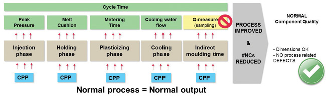
The injection molding process was divided into phases and for each phase, PIs (green) and CPPs (blue) were found as shown in Figure 2. The DoE established relationships between CPPs, PIs and CQAs (dimensions and defects). Based on these relationships, product testing has been replaced by in-line release testing of PIs.

The major outcomes of implementing in-line release testing have been:

• Significantly reduced risk of approving random errors
• Validation time reduced from 20 weeks to three weeks
• Scrap rate reduced 70%
• Overall equipment effectiveness increased 7%

Case Study 2: Process Optimization

A manufacturer experienced yield issues after upscaling. The first 11 pilot runs after upscaling were analyzed for correlations between yield, PIs and CPPs. The challenge here was that CPPs (e.g., feed) and PIs (e.g., glucose consumption and lactate production) were functions of time as shown in Figure 3.

This issue was solved using the functional data explorer in JMP software from SAS. Functional principal components (FPC) of curve fits were used to describe the curves. Relationships between yield and PI FPCs were found using partial least squares modelling (due to heavily correlated PIs) and standard least squares modeling to establish relationships between PIs and CPPs. The combined relationships are shown in the Figure 4, namely, how the optimal PI curves were obtained by changing the CPPs.

By following this process, the manufacturer increased the average yield by 30% and reduced yield variation from batch to batch by 70%.

                

                

Conclusion

Continuous process control has many advantages compared to continued product verification. By conducting continuous verification there is a low risk of overlooking errors compared to traditional sampling. Knowing the relationships between CQAs and PIs forms the basis for real-time release testing. Process control is an active operation; process parameters are adjusted to keep process quality on target as opposed to process verification where it is only verified to be within specification.

Robust manufacturing processes result from processes kept on target instead of merely just inside specifications. Continuous process control is also a prerequisite for continuous processing, which is becoming popular due to the smaller footprint, shorter processing times and increased flexibility.